Transfering Style!
Original Notebook : https://www.kaggle.com/code/ohseokkim/transfering-style
Introduction
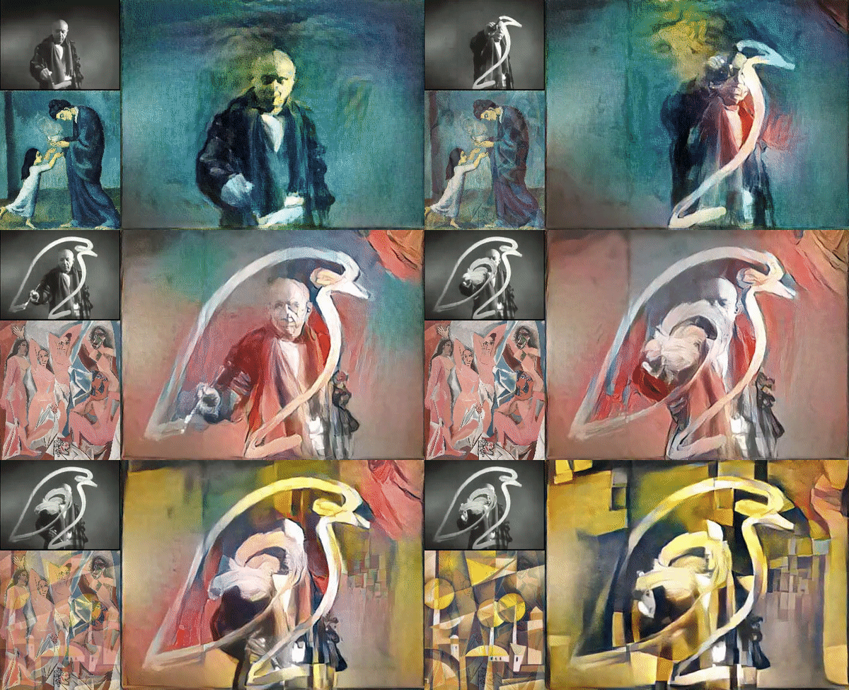 Picture Credit: https://miro.medium.com
Nearal Style Transfer
Neural Style Transfer(NST) refers to a class of software algorithms that manipulate digital images, or videos, in order to adopt the appearance or visual style of another image. NST algorithms are characterized by their use of deep neural networks for the sake of image transformation. Common uses for NST are the creation of artificial artwork from photographs, for example by transferring the appearance of famous paintings to user-supplied photographs. Several notable mobile apps use NST techniques for this purpose, including DeepArt and Prisma. This method has been used by artists and designers around the globe to develop new artwork based on existent style(s).
Style transfer means that when a content image and a style image are given, the outline and shape of the image are similar to the content image, and the color or texture is changed to be similar to the style image.
By separating content and style, you can mix content and style of different images.
A pre-trained VGG19 Net is used as model to extract content and style. It then uses the losses of the content and style to iteractively update the target image until the desired result is achieved.
from PIL import Image
from io import BytesIO
import matplotlib.pyplot as plt
import numpy as np

import torch
import torch.optim as optim
import requests
from torchvision import transforms, models
1. Load in model
VGG19 is divided into two parts.
- vgg19.features: All convolutional layers and pooling layers
- vgg19.classifier: The last three linaer layers are the classifier layer.
We only need the features part. And “freeze” so that the weight is not updated.
# get the "features" portion of VGG19 (we will not need the "classifier" portion)
with HiddenPrints():
  vgg = models.vgg19(weights="IMAGENET1K_V1").features

  # freeze all VGG parameters since we're only optimizing the target image
  for param in vgg.parameters():
    param.requires_grad_(False)
# move the model to GPU, if available
device = torch.device("cuda" if torch.cuda.is_available() else "cpu")

vgg.to(device)
#> Sequential(
#>   (0): Conv2d(3, 64, kernel_size=(3, 3), stride=(1, 1), padding=(1, 1))
#>   (1): ReLU(inplace=True)
#>   (2): Conv2d(64, 64, kernel_size=(3, 3), stride=(1, 1), padding=(1, 1))
#>   (3): ReLU(inplace=True)
#>   (4): MaxPool2d(kernel_size=2, stride=2, padding=0, dilation=1, ceil_mode=False)
#>   (5): Conv2d(64, 128, kernel_size=(3, 3), stride=(1, 1), padding=(1, 1))
#>   (6): ReLU(inplace=True)
#>   (7): Conv2d(128, 128, kernel_size=(3, 3), stride=(1, 1), padding=(1, 1))
#>   (8): ReLU(inplace=True)
#>   (9): MaxPool2d(kernel_size=2, stride=2, padding=0, dilation=1, ceil_mode=False)
#>   (10): Conv2d(128, 256, kernel_size=(3, 3), stride=(1, 1), padding=(1, 1))
#>   (11): ReLU(inplace=True)
#>   (12): Conv2d(256, 256, kernel_size=(3, 3), stride=(1, 1), padding=(1, 1))
#>   (13): ReLU(inplace=True)
#>   (14): Conv2d(256, 256, kernel_size=(3, 3), stride=(1, 1), padding=(1, 1))
#>   (15): ReLU(inplace=True)
#>   (16): Conv2d(256, 256, kernel_size=(3, 3), stride=(1, 1), padding=(1, 1))
#>   (17): ReLU(inplace=True)
#>   (18): MaxPool2d(kernel_size=2, stride=2, padding=0, dilation=1, ceil_mode=False)
#>   (19): Conv2d(256, 512, kernel_size=(3, 3), stride=(1, 1), padding=(1, 1))
#>   (20): ReLU(inplace=True)
#>   (21): Conv2d(512, 512, kernel_size=(3, 3), stride=(1, 1), padding=(1, 1))
#>   (22): ReLU(inplace=True)
#>   (23): Conv2d(512, 512, kernel_size=(3, 3), stride=(1, 1), padding=(1, 1))
#>   (24): ReLU(inplace=True)
#>   (25): Conv2d(512, 512, kernel_size=(3, 3), stride=(1, 1), padding=(1, 1))
#>   (26): ReLU(inplace=True)
#>   (27): MaxPool2d(kernel_size=2, stride=2, padding=0, dilation=1, ceil_mode=False)
#>   (28): Conv2d(512, 512, kernel_size=(3, 3), stride=(1, 1), padding=(1, 1))
#>   (29): ReLU(inplace=True)
#>   (30): Conv2d(512, 512, kernel_size=(3, 3), stride=(1, 1), padding=(1, 1))
#>   (31): ReLU(inplace=True)
#>   (32): Conv2d(512, 512, kernel_size=(3, 3), stride=(1, 1), padding=(1, 1))
#>   (33): ReLU(inplace=True)
#>   (34): Conv2d(512, 512, kernel_size=(3, 3), stride=(1, 1), padding=(1, 1))
#>   (35): ReLU(inplace=True)
#>   (36): MaxPool2d(kernel_size=2, stride=2, padding=0, dilation=1, ceil_mode=False)
#> )
2. Load in Content and Style Images
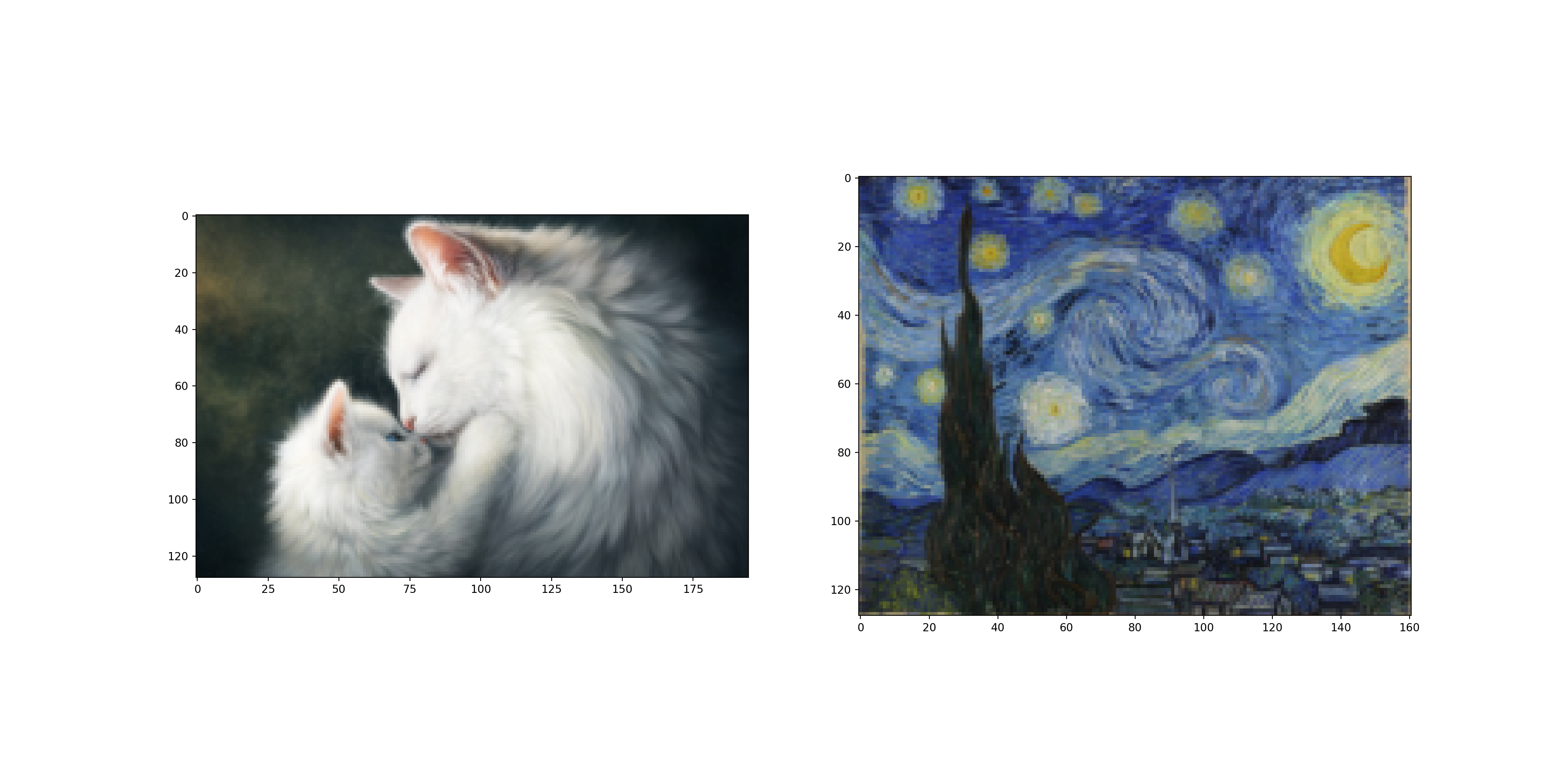
Load the content image and style image to be used for style transfer. The load_image function transforms the image and loads it in the form of normalized Tensors.
def load_image(img_path, max_size = 128, shape = None):
  '''
  Load in and transform an image, making sure the image is <= 400 pixels in the x-y dims.
  '''

  if "http" in img_path:
    response = requests.get(img_path)
    image = Image.open(BytesIO(response.content)).convert('RGB')
  else:
    image = Image.open(img_path).convert('RGB')

  # large images will slow down processing
  if max(image.size) > max_size:
    size = max_size
  else:
    size = max(image.size)

  if shape is not None:
    size = shape

  in_transform = transforms.Compose([
    transforms.Resize(size),
    transforms.ToTensor(),
    transforms.Normalize((0.485, 0.456, 0.406), (0.229, 0.224, 0.225))
  ])

  # discard the transparent, alpha channel (that's the :3) and add the batch dimension
  image = in_transform(image)[:3, :, :].unsqueeze(0)

  return image
# load in content and style image
content = load_image("./data/856047.jpg").to(device)
# Resize style to match content, makes code easier
style = load_image("./data/starry_night.jpg").to(device)
# helper function for un-normalizing an image
# and converting it from a Tensor image to a NumPy image for dispaly
def im_convert(tensor):
  """
  Display a tensor as an image.
  """

  image = tensor.to("cpu").clone().detach()
  image = image.numpy().squeeze()
  image = image.transpose(1, 2, 0)
  image = image * np.array((0.229, 0.224, 0.225)) + np.array((0.485, 0.456, 0.406))
  image = image.clip(0, 1)

  return image
#display the images
fig, (ax1, ax2) = plt.subplots(1, 2, figsize = (20, 10))
# content and style ims side-by-side
ax1.imshow(im_convert(content))
ax2.imshow(im_convert(style))

plt.show()
def get_features(image, model, layers = None):
  """
  Run an image forward through a model and get the features for a set of layers. Default layers are for
  VGGNet matching Gatys et al (2016)
  """

  if layers is None:
    layers = {'0' : 'conv1_1',
              '5' : 'conv2_1',
              '10': 'conv3_1',
              '19': 'conv4_1',
              '21': 'conv4_2', ## content representation
              '28': 'conv5_1'}

  features = {}
  x = image
  # model._modules is a dictionary holding each module in the model
  for name, layer in model._modules.items():
    x = layer(x)
    if name in layers:
      features[layers[name]] = x

  return features
3. Gram Matrix
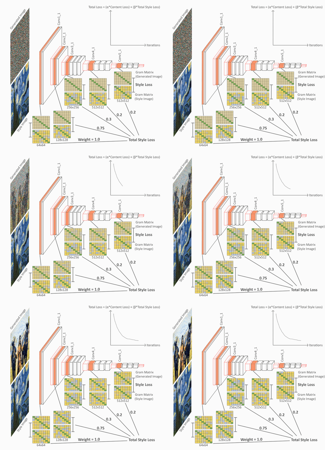 Picture Credit: https://miro.medium.com
The matrix expressing the correlation of this Channel is called Gram Matrix. Loss is minimized by definding the difference between this Gram Matrix and the Gram Matrix of the newly created image as a Loss Function. Next, in order to reflect the content, the loss function is calculated in units of pixels from the feature map spit out from each pre-trained CNN. In this way, a new image is created that minimizes the Loss calculated from Style and Loss calculated from Content.
https://en.wikipedia.org/wiki/Gram_matrix
def gram_matrix(tensor):
  """
  Calculate the Gram Matrix of a given tensor
  """

  # get the batch_size, depth, height, and width of the Tensor
  _, d, h, w = tensor.size()

  # reshape so we're multiplying the features for each channel
  tensor = tensor.view(d, h * w)

  # calculate the gram matrix
  gram = torch.mm(tensor, tensor.t())

  return gram
The function that extracts the features of a given convolutional layer and computes the Gram Matrix is made. Putting it all together, we extract the features from the image and compute the Gram Matrix for each layer from the style representation.
# get content and style features only once before training
content_features = get_features(content, vgg)
style_features = get_features(style, vgg)

# calculate the gram matrices for each layer of our style representation
style_grams = {layer: gram_matrix(style_features[layer]) for layer in style_features}

# create a third "target"image and prep it for change
# it is a good idea to start off with the target as a copy of our *content* image
# then iteratively change its style
target = content.clone().requires_grad_(True).to(device)
4. Define Losses and Weights
Individual Layer Style Weights
You can give the option to weight the style expression in each relevant layer. It is recommended that the layer weight range from 0 to 1. By giving more weight to conv1_1 and conv2_1, more style artifacts can be reflected in the final target image.
Content and Style Weight
Define alpha (content_weight) and beta (style_weight). This ratio affaects the style of the final image. It is recommended to leave content_weight = 1 and set style_weight to achieve the desired ratio.
# weights for each style layer
# weighting ealier layers more will result in *larger* style artifacts
# notice we are excluding `conv4_2` our content representation
style_weights = {'conv1_1' : 1,
                 'conv2_1' : 0.75,
                 'conv3_1' : 0.2,
                 'conv4_1' : 0.2,
                 'conv5_1' : 0.2}

content_weight = 1 # alpha
style_weight = 1e3 # beta
5. Update Target and Calculate Losses
Content Loss
The Content loss is calculated as the MSE between the target and the content feature in the ‘conv4_2’ layer.
Style Loss
The style loss is the loss between the target image and the style image. That is, it refers to the difference between the gram matrix of the style image and the gram matrix of the target image. Loss is calculated using MSE
Total Loss
Fianlly, the total loss is calculated by summing the style and content losses and weighting them with the specified alpha and beta.
# for displaying the target image, intermittently
show_every = 500

# iteration gyperparameters
optimizer = optim.Adam([target], lr = 0.003)
steps = 5001 # decide how many iterations to update your image (5000)

for ii in range(1, steps+1):

  # get the features from your target image
  target_features = get_features(target, vgg)

  # the content loss
  content_loss = torch.mean((target_features['conv4_2'] - content_features['conv4_2'])**2)

  # the style loss
  # initialize the style loss to 0
  style_loss = 0
  # then add to it for each layer's gram matrix loss
  for layer in style_weights:
    # get the "target" style representation for the layer
    target_feature = target_features[layer]
    target_gram    = gram_matrix(target_feature)
    _, d, h, w = target_feature.shape
    # get the "style" style representation
    style_gram = style_grams[layer]
    # the style loss for one layer, weighted appropriately
    layer_style_loss = style_weights[layer] * torch.mean((target_gram - style_gram) ** 2)
    # add to the style loss
    style_loss += layer_style_loss / (d * h * w)

  # calculate the *total* loss
  total_loss = content_weight * content_loss + style_weight * style_loss

  # update your target image
  optimizer.zero_grad()
  total_loss.backward()
  optimizer.step()

  # display intermediate images and print the loss
  if ii % show_every == 0:
    print('Total loss: ', total_loss.item())
    plt.imshow(im_convert(target))
    plt.show()
#> Total loss:  812.097900390625
#> <matplotlib.image.AxesImage object at 0x7fe0cdeabd90>
#> Total loss:  498.1385498046875
#> <matplotlib.image.AxesImage object at 0x7fe0cd537e80>
#> Total loss:  365.70355224609375
#> <matplotlib.image.AxesImage object at 0x7fe0cded2620>
#> Total loss:  290.7293395996094
#> <matplotlib.image.AxesImage object at 0x7fe0cd5ceb00>
#> Total loss:  243.23556518554688
#> <matplotlib.image.AxesImage object at 0x7fe0cd4494e0>
#> Total loss:  210.29429626464844
#> <matplotlib.image.AxesImage object at 0x7fe0cd4d0700>
#> Total loss:  186.3564910888672
#> <matplotlib.image.AxesImage object at 0x7fe0cd34f0a0>
#> Total loss:  168.50942993164062
#> <matplotlib.image.AxesImage object at 0x7fe0cd3afa00>
#> Total loss:  154.83030700683594
#> <matplotlib.image.AxesImage object at 0x7fe0cd49f9a0>
#> Total loss:  143.84054565429688
#> <matplotlib.image.AxesImage object at 0x7fe0cd34c1c0>
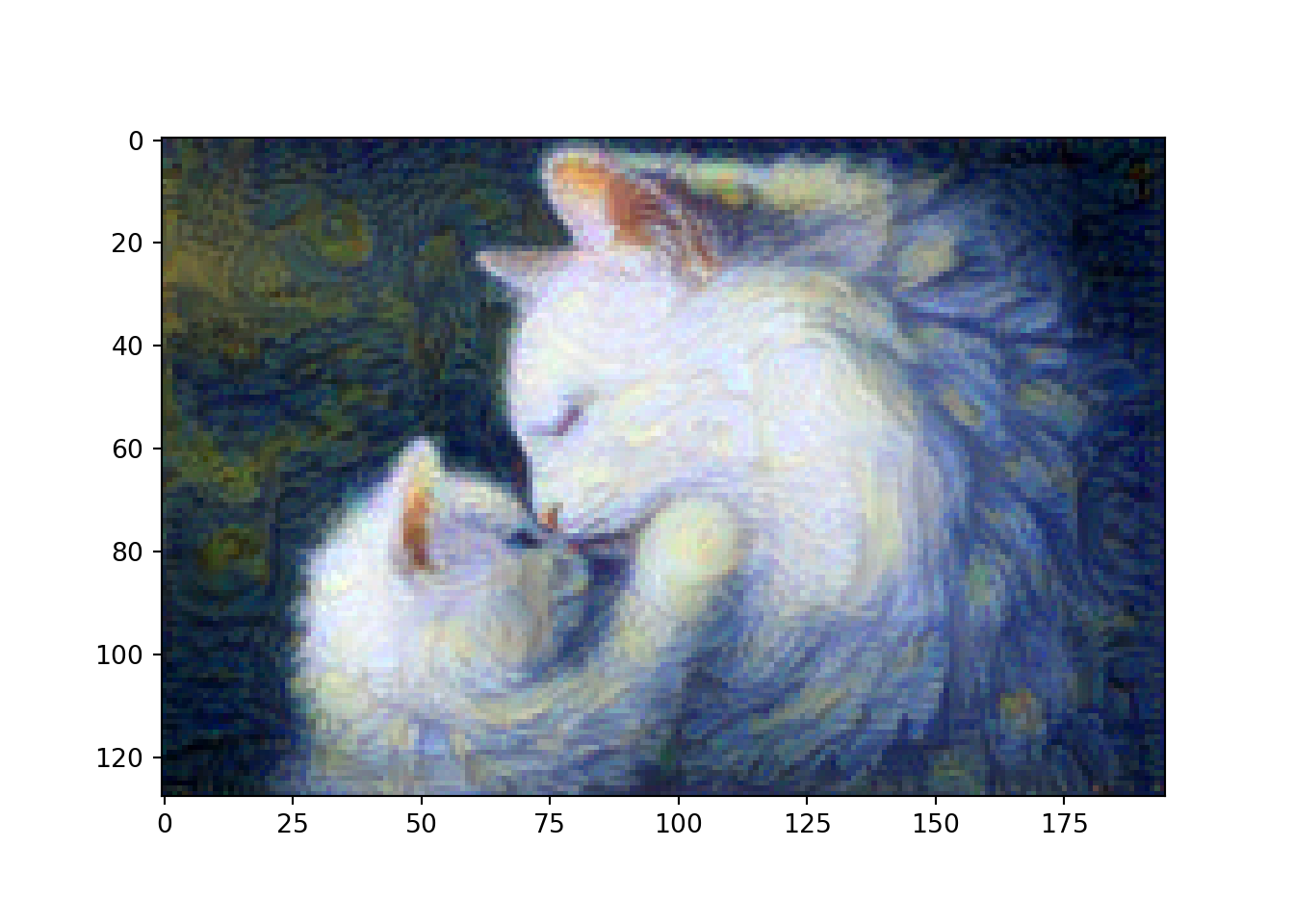
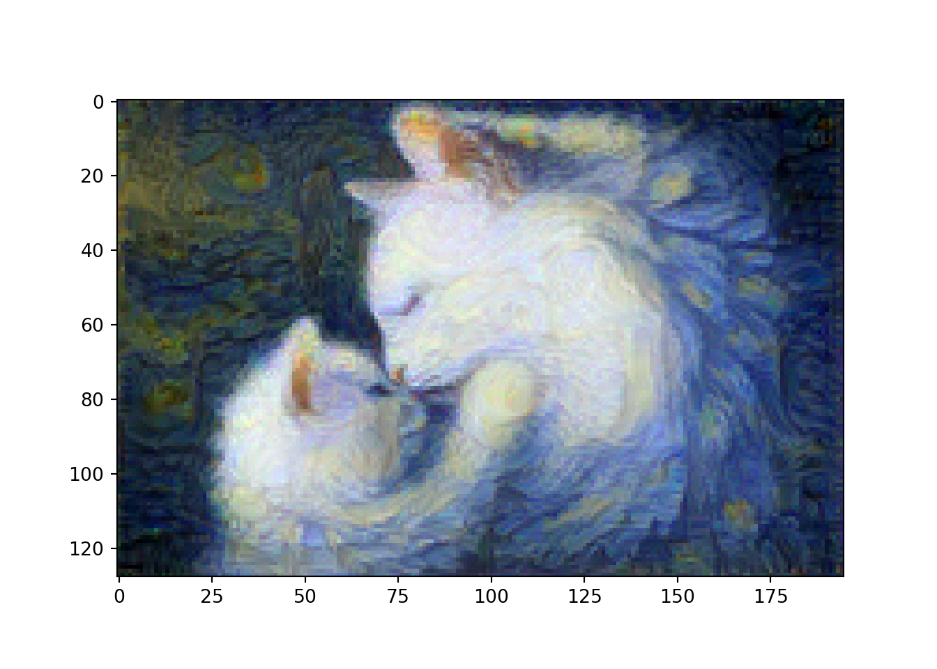

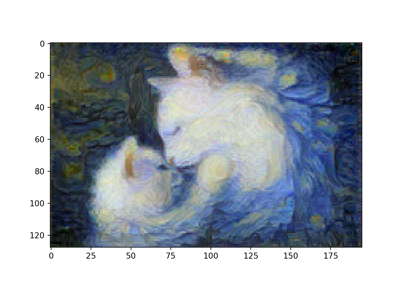


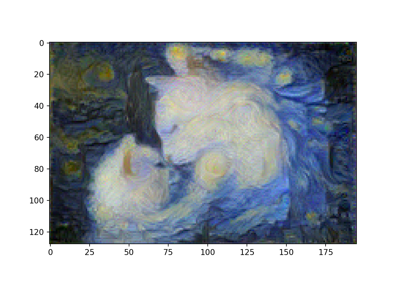
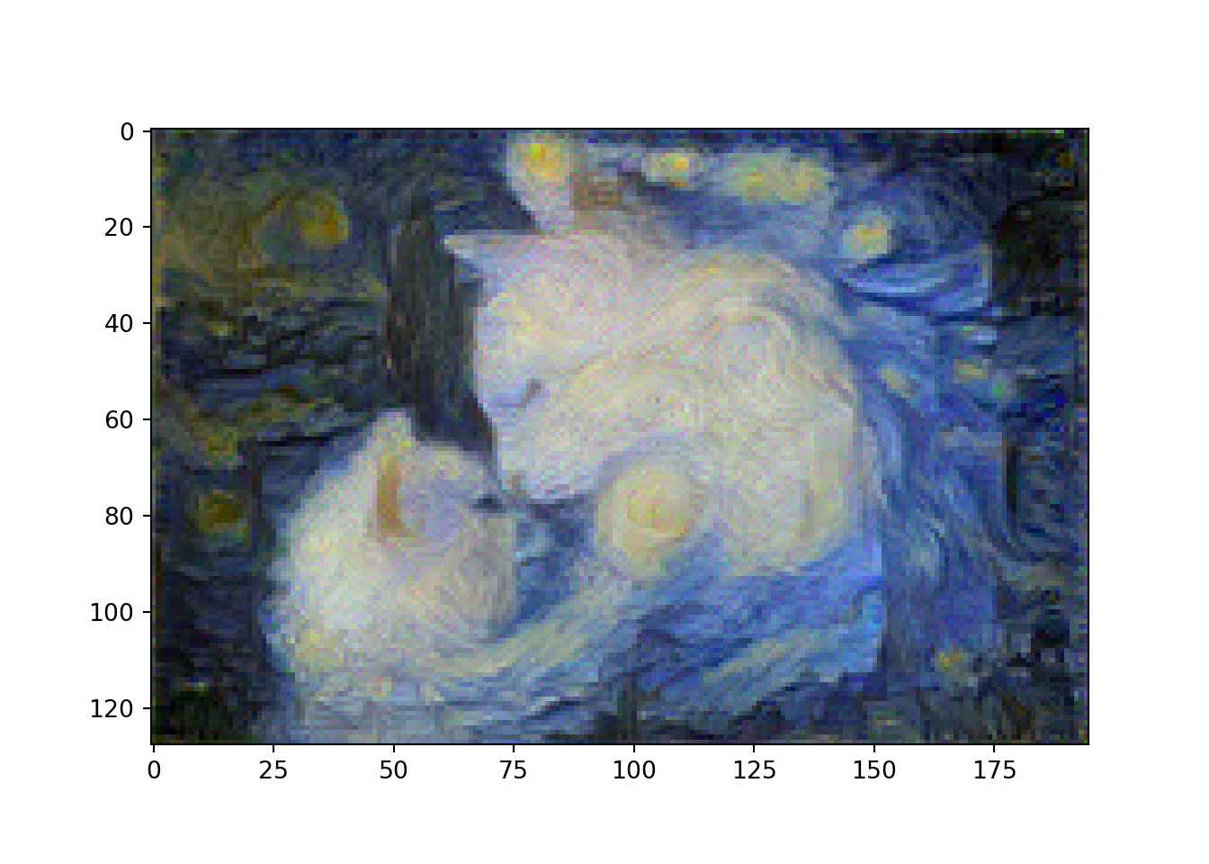
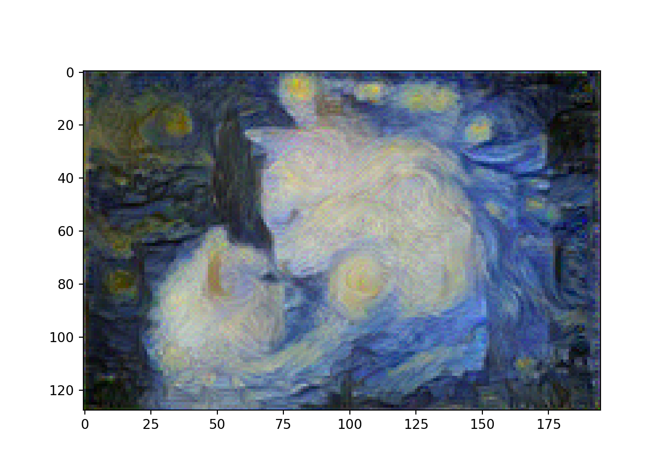

6. Check the last result
# display content and final, target image
fig, (ax1, ax2) = plt.subplots(1, 2, figsize = (20, 10))
ax1.imshow(im_convert(content))
#> <matplotlib.image.AxesImage object at 0x7fe0cd47a4d0>
ax2.imshow(im_convert(target))
#> <matplotlib.image.AxesImage object at 0x7fe0cd47bd30>
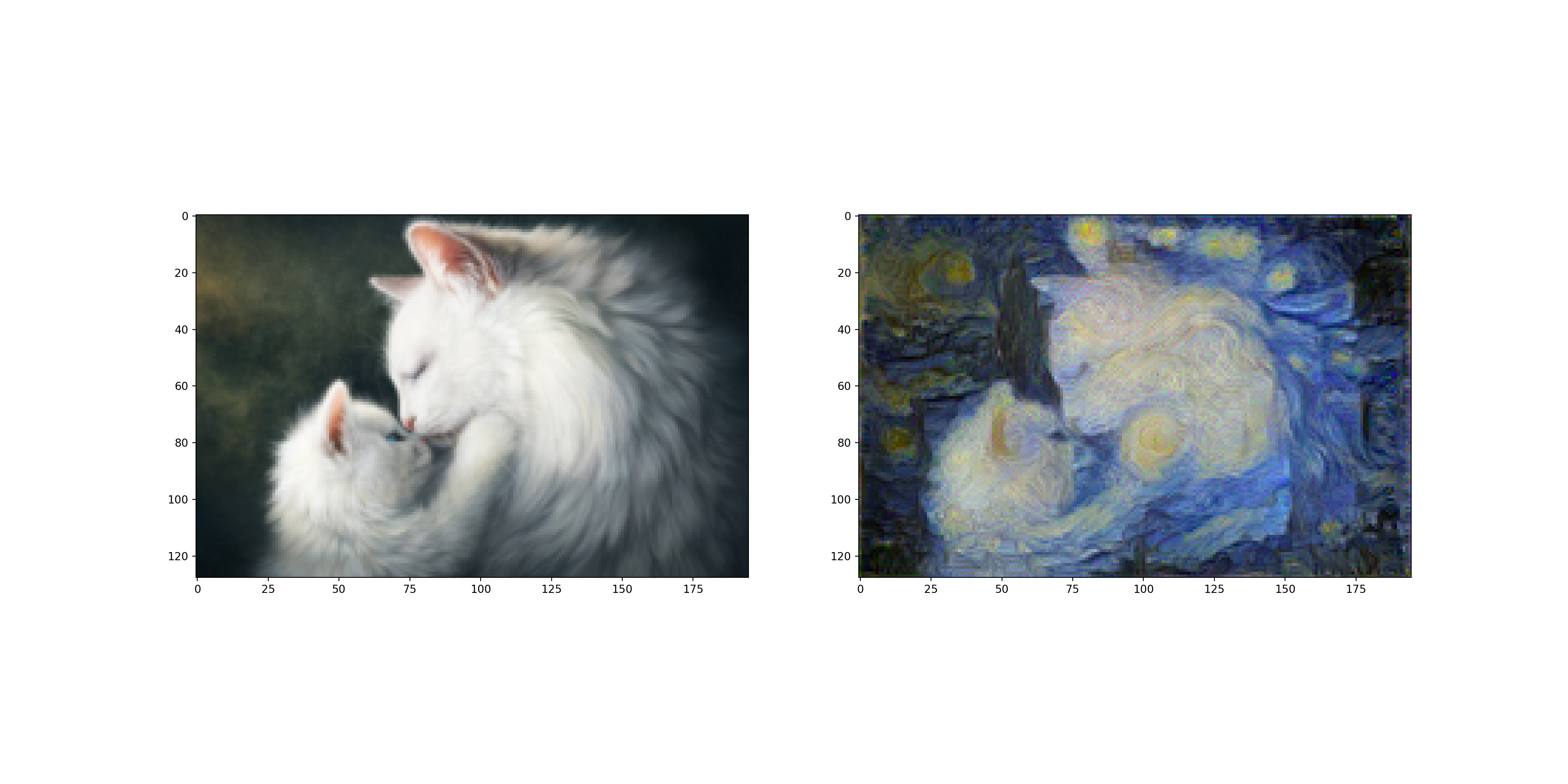
plt.show()
